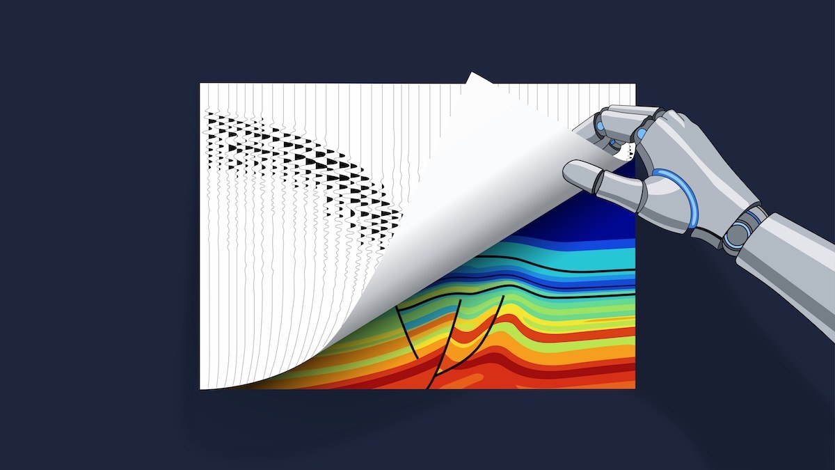
Full-waveform inversion (FWI) is a notoriously ill-posed inverse problem. We replace its hand-crafted regularizer with the gradient of a pretrained diffusion model — a trick borrowed from the Regularization-by-Denoising (RED) literature. The result is plug-and-play, generalizes across geological datasets it was never trained on, and beats TV / Tikhonov baselines on SSIM, MAE and RMSE.
Seismic imaging asks a question that sounds simple and is not: given a few seconds of pressure recorded on the surface of the Earth, what does the subsurface look like? The forward problem — propagating an acoustic wave through a known velocity field — is governed by a linear PDE we understand well. The inverse problem is where things get interesting.
Full-waveform inversion (FWI) is the workhorse method: pose the question as an optimization, minimize the mismatch between observed and simulated seismograms, and let gradient descent find a velocity field that explains the data. In practice the loss surface is non-convex, the data is band-limited, noise is everywhere, and there are infinitely many velocity models that fit the data almost equally well. Without a strong prior on what an Earth model is supposed to look like, FWI happily lands in geologically implausible minima.
01The setup
Let $m \in \mathbb{R}^{H \times W}$ be a 2D velocity model of the subsurface, and $d_{\text{obs}}$ the observed seismic recording. The forward operator $\mathcal{F}$ solves the acoustic wave equation,
and samples the wavefield $u$ at receiver locations to produce a simulated shot record. FWI then minimizes the data misfit
If equation (2) were the whole story, life would be easy and seismologists would be bored. Two facts make it hard: non-uniqueness — many wildly different $m$ produce nearly identical $\mathcal{F}(m)$ — and non-convexity, where the optimizer settles in a local minimum that fits the data but looks nothing like rock.
The standard fix is to add a regularizer $R(m)$ that penalizes models we believe are unphysical:
Tikhonov sets $R(m) = \|\nabla m\|_2^2$ (smoothness). Total variation sets $R(m) = \|\nabla m\|_1$ (piecewise-constant blocks with sharp edges). Both encode a single, hand-picked belief about the world. Real geology — folded layers, faults, salt bodies — is more nuanced than either.
02What if the regularizer were a neural network?
The Regularization-by-Denoising (RED) framework, due to Romano, Elad and Milanfar, observes something striking: if you have a good denoiser $D_\sigma$ — a function that maps noisy images to clean ones — you can plug it into an inverse problem as if it were the gradient of a regularizer, via the update
The interpretation is lovely: at each step, nudge the current estimate toward what the denoiser thinks it should look like. The denoiser carries the prior; we never write it down by hand.
What's the best denoiser we have? A score-based diffusion model. The score function $\nabla_x \log p_t(x)$ learned during diffusion training is, up to scaling, exactly a denoiser — Tweedie's formula gives $\mathbb{E}[m_0 \mid m_t] = m_t + \sigma_t^2\, \nabla_{m_t}\log p_t(m_t)$. So a diffusion model trained on synthetic velocity models from OpenFWI gives us $D_\sigma$ for free, at every noise level. RED-DiffEq plugs that into FWI.
The diffusion model never sees seismic data. It only learns what subsurfaces look like — and that turns out to be enough.
03The RED-DiffEq update
Putting the pieces together, the RED-DiffEq objective is $\min_x \tfrac{1}{2}\|f_{\text{PDE}}(x) - u_{\text{obs}}\|_2^2 + \lambda\, R_{\text{diff}}(x)$. The regularizer is the score-matching residual at a freshly-sampled noise level,
with $t \sim \mathcal{U}\{1,\dots,T\}$ and $\varepsilon \sim \mathcal{N}(0, \mathbf{I})$ drawn fresh at every iteration. The stop-gradient $\mathrm{sg}$ treats the network’s prediction as a constant w.r.t. $x$, so the regularization gradient collapses to the noise-prediction residual $\varepsilon_\theta(x_t, t) - \varepsilon$. The full objective gradient is therefore
The first term is the standard FWI gradient — an adjoint-state solve of the wave equation. The second is the noise-prediction error of the frozen diffusion network on a freshly-noised copy of the current iterate: stochastic in $t$ and $\varepsilon$, deterministic in everything else. No Langevin sampling, no posterior MCMC, no retraining on seismograms.
04Does it work?
We train the diffusion model on horizontally-layered velocity models from OpenFWI — the simpler geology in the corpus — then deploy that same prior, with no fine-tuning, on in-domain OpenFWI data and on two out-of-distribution benchmarks: Marmousi and Overthrust, both structurally complex. Baselines: physics-driven FWI, FWI + Tikhonov, FWI + total variation, and two diffusion-based competitors. We also push every method through Gaussian noise, Laplacian noise, and missing traces.
Schematic reconstructions on a synthetic folded cross-section. FWI smears the fine detail; TV introduces blocky artifacts; RED-DiffEq recovers the folded structure. Illustrative — see the paper for quantitative SSIM / MAE / RMSE results.
The qualitative picture: FWI alone gets the broad strokes but smears the high-wavenumber detail. Tikhonov over-smooths, blurring out faults. TV gives blocky, cartoon-like reconstructions. RED-DiffEq recovers the structural geometry — folded layers, fault offsets — and, crucially, its error curves stay flat as the data degrades: the prior keeps the inversion honest when the measurements are not.
05Why does the cross-dataset transfer work?
This is the most interesting finding. The diffusion model has only ever seen relatively simple layered geology, yet the prior it provides is useful for folded thrust geology it never trained on.
Our hypothesis: the denoiser doesn't encode specific geological structures so much as a local statistical signature of what subsurface velocity fields look like — piecewise smooth with sharp velocity contrasts, anisotropic correlation lengths, particular noise statistics. Those local statistics stay remarkably consistent across geological families even when the global structure changes dramatically. The RED gradient pushes toward them without ever committing to a specific topology.
Said another way: TV says "the world is piecewise constant." Tikhonov says "the world is smooth." The diffusion prior says "the world looks like this" — a much richer, structurally-correct claim, even on data it wasn't trained on.
06Limitations & what's next
The honest list: the method is 2D and acoustic, while real seismic is 3D and elastic; the noise level $\sigma_t$ remains a knob that wants a principled annealing schedule; and we benchmark on synthetic data with known ground truth, so real field recordings will stress the prior's tails harder.
Next, I want to replace the explicit RED gradient with a properly-derived posterior-sampling scheme, port the framework to elastic FWI, and ask whether the same trick — pretrained generative prior, no posterior sampling, plug into an existing PDE-constrained pipeline — works for other scientific inverse problems. Optical tomography and electrical impedance tomography are obvious candidates.
07Cite
- Shan, S., Zhu, M., Lin, Y., & Lu, L. Regularization by denoising diffusion models for solving inverse PDE problems with application to full waveform inversion. Communications Physics (2026). DOI: 10.1038/s42005-026-02677-6.
- Romano, Y., Elad, M., & Milanfar, P. The little engine that could: Regularization by denoising (RED). SIAM Journal on Imaging Sciences, 10(4), 2017.
- Ho, J., Jain, A., & Abbeel, P. Denoising diffusion probabilistic models. NeurIPS 2020.
- Deng, C. et al. OpenFWI: Large-scale multi-structural benchmark datasets for full waveform inversion. NeurIPS Datasets & Benchmarks 2022.